Rakeness

• IntroductionIntroduction
• DefinitionDefinition
• ExamplesExample
• More detailsMore details

Compressed Sensing (CS) is a technique that allows the reconstruction of signals starting from a limited number of linear measurements that is potentially much smaller than the number of Nyquist-rate samples. The possibility of such sub-Nyquist representation hinges on an assumption on the considered class of signals, i.e., that they are sparse. To model signals and the sparsity assumption we may think to collect the signal samples from a given time window in the \(n\)-dimensional vector \(x\in\mathbb{R}^n\) and consider its representation w.r.t. a set of vectors arranged as the columns of a matrix \(S\). It is commonly assumed that the set of vectors spans the whole \(\mathbb{R}^n\) though it may be redundant and contain more than \(n\) vectors. For simplicity's sake we here assume that there is no redundancy and thus that \(S\) is a base. With this we know that \(x=S\xi\) with \(\xi=S^{-1}x\) and \(x\) is said to be \(\kappa\)-sparse if \(\xi\) has at most \(\kappa\) non-zero components with \(\kappa\ll n\).

If this happens the actual number of degrees of freedom in \(x\) is smaller than \(n\). Thus, the signal information content can be represented by a measurement vector \(y\in\mathbb{R}^m\) obtained by projections on a proper set of sensing vectors arranged as rows of the sensing matrix \(A\). $$ y = Ax =A S \xi $$ If \(m \lt n\) measuraments are enough to capture the needed signal information content then a signal compression is achieved with a corresponding compression ratio defined as \(CR = \frac{n}{m}\).

If the matrix \(AS\) satisfies certain conditions, \(\xi\) (and thus \(x\)) can be recovered from \(y\) despite the fact that \(A\) (and thus \(A S\)) is a dimensionality reduction, provided that \(m = \mathcal{O}(\kappa \log n)\). This hints to the fact that non-negligible values of \(CR\) may be obtained. Roughly speaking, the conditions on \(AS\) require that generic \(\kappa\)-sparse vectors are mapped almost-isometrically into the measurements. Such conditions are commonly satisfied by setting \(A\) as an instance of a random matrix with independent and identically distributed entries, Gaussian or Bernoulli distributions being the most commonly adopted. Once this is done, \(x\) is computed from \(y = A x\) by enforcing the a priori knowledge that its representation \(\xi\) is sparse. Algorithmically, the sparse signal recovery can be obtained by solving of the following convex optimization problem $$ \begin{array}{c} \displaystyle\hat{x}=\arg\left\{\min_{\zeta}\|S^{-1} \zeta\|_{1}\right\}\\ \text{s.t.}\;\; \|A \zeta -y\|^2_2 \le \epsilon^2 \end{array} $$ where \(\|S^{-1} \zeta\|_{1}\) is a sparsity-promoting norm, i.e., a quantity that decreases as the representation of the signal w.r.t. the basis \(S\) conforms with the sparsity prior, and \( \|A \zeta -y\|^2_2\) is the usual Euclidean norm that measures the accuracy with which the measurements \(y\) are matched by the solution. The parameter \(\epsilon\ge 0\) is chosen proportionally to the amount of noise affecting \(y\), \(\epsilon = 0\) corresponding to the noiseless case.

Donoho, D.L., "Compressed sensing," Information Theory, IEEE Transactions on, vol.52, no.4, pp.1289-1306, 2006 - doi: 10.1109/TIT.2006.871582

Candes, E.J.; Wakin, M.B., "An Introduction To Compressive Sampling," Signal Processing Magazine, IEEE, vol.25, no.2, pp.21-30, 2008 - doi: 10.1109/MSP.2007.914731

Haboba, J.; Mangia, M.; Pareschi, F.; Rovatti, R.; Setti, G., "A Pragmatic Look at Some Compressive Sensing Architectures With Saturation and Quantization," Emerging and Selected Topics in Circuits and Systems, IEEE Journal on, vol.2, no.3, pp.443-459, 2012 - doi: 10.1109/JETCAS.2012.2220392

The general CS theory does not depend on the specific class of signals to acquire, and claims of universality are quite frequent in the Literature. Yet, from a purely engineering perspective, whenever degrees of freedom and a priori knowledge on the application are simultaneously present, the obvious way to go is to use available knobs to optimize the system. To this end, one may note that most of the practical interest in CS comes from two key facts:

• Although theoretical upper bounds exist on the error committed by signal recovery algorithms, real performances are typically much better than those predicted by formal guarantees, yielding extremely effective signal acquisition.
• The mathematical conditions that allow signal recovery algorithms to succeed can be matched (with very high probability) by simply drawing \(A\) at random. Although theoretical guarantess deped on the choiche of specific distributions, in practice a wide class of random matrices allow for effective recovery.

Starting from these considerations, one may adjust the statistical distribution of \(A\) to optimize the acquisition performance depending on the actual statistics of the signal \(x\). This is what the rakeness approach does, yielding a random policy for drawing \(A\) that increases the CS performance either by reducing the minimum \(m\) nedeed for a correct reconstruction or by improving reconstruction quality for a fixed \(m\).

More specifically, one exploits the fact that in real-world applictions, the input vectors are usually not only sparse but also non-white or localized, i.e., their energy content is not uniformly distributed in the whole signal space. The idea is to choose the generic sensing matrix row \(a=(a_1,\dots,a_n)\) so to increase the average energy collected (i.e., “raked”) when the input signal is projected onto it, preserving at same time the randomness of \(A\) that allows to expect a satisfactory reconstruction in all cases.

Formally, let us model \(a\) and \(x\) as realizations of two independent stochastic processes whose \(n\times n\) correlation matrices are given by \(\mathcal{A}=\mathbf{E}[aa^\top]\) and \(\mathcal{X}=\mathbf{E}[xx^\top]\). We define rakeness the average energy of the projection of \(x\) on \(a\), i.e., the quantity $$ \begin{array}{rcl} \rho(a,x)& =& \mathbf{E}[(a^\top x)^2]=\mathbf{E}[a^\top x x^\top a]\\ &=&\mathbf{E}[a^\top\mathcal{X}a]=\mathbf{E}[{\rm tr}(aa^\top\mathcal{X})]\\ &=&{\rm tr}(\mathcal{A}\mathcal{X})=\sum_{i=1}^{n}\sum_{j=1}^n \mathcal{A}_{i,j}\mathcal{X}_{i,j} \end{array} $$ Clearly, \(\rho\) is a measure of average alignment between random vectors. Actually, it can be also used to measure the whiteness of the distribution of a random vector since this last concept is related to the average aligment between any pair of vectors drawn independently from such a distribution. Hence, \(\rho(a,a)={\rm tr}(\mathcal{A}^2)=\sum_{j=1}^n\sum_{j=1}^n(\mathcal{A}_{i,j})^2\) can be bounded from above to guarantee that the sensing row is distributed in a sufficiently isotropic way.

Rakeness-based design aims at maximizing the ability of the projections of collecting the signal energy while keeping them random enough to span the signal space. This is mapped into the following optimization problem: $$ \begin{array}{ll} \displaystyle \max_{\mathcal{A}} & \;\;\displaystyle \mathrm{tr}(\mathcal{A}\mathcal{X})\\[0.5em] {\rm s.t.} & \begin{array}{l} \mathcal{A}\succeq 0\\ \mathrm{tr}(\mathcal{A})=e\\ \rho(a,a)=\mathrm{tr}(\mathcal{A}^2)\le \tau e^2 \end{array} \end{array} $$ where \(\mathcal{A}\succeq 0\) indicates the need for a positive semi-definite \(\mathcal{A}\), the energy of each row (\({\rm tr(\mathcal{A})}=\sum_{i=1}^n\mathcal{A}_{i,i}\)) is normalized to a certain \(e\), and \(\tau\le 1\) controls the strength of the randomness constraint. Tuning of \(\tau\) on a proper and known range is not critical (see Bertoni 2013), since it does not appreciably alter the overall system performance. The solution of this optimization problem (given in analytical terms in Mangia 2012) yields a correlation matrix \(\mathcal{A}\), that identifies the stochastic process to be used for generating sensing vectors.

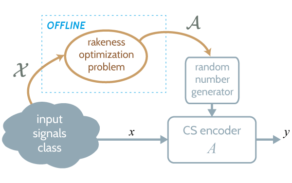
The following picture sketches the rakeness-based design flow. For a given input signal class, i.e., a given \(\mathcal{X}\), the matrix \(\mathcal{A}\) is computed offline. After that, the whole sensing process works without any additional processing with respect to a standard CS encoder. Applying rakeness only means use sensing vectors with an optimized correlation profile in place of purely random ones.

It has been demonstrated (see references below) that exploiting rakeness-based design means increasing the quality of the reconstructed signal for a given value of \(m\), or, viceversa, decreasing the minimum \(m\) guaranteeing a prescribed reconstruction quality.

Mangia, M.; Rovatti, R.; Setti, G., "Rakeness in the Design of Analog-to-Information Conversion of Sparse and Localized Signals," Circuits and Systems I: Regular Papers, IEEE Transactions on, vol.59, no.5, pp.1001-1014, 2012 - doi: 10.1109/TCSI.2012.2191312

Bertoni, N.; Mangia, M.; Pareschi, F.; Rovatti, R.; Setti, G., "Correlation tuning in compressive sensing based on rakeness: A case study," Electronics, Circuits, and Systems (ICECS), 2013 IEEE 20th International Conference on, pp.257-260, 2013 - doi: 10.1109/ICECS.2013.6815403

Mangia, M.; Rovatti, R.; Setti, G., "Analog-to-information conversion of sparse and non-white signals: Statistical design of sensing waveforms," Circuits and Systems (ISCAS), 2011 IEEE International Symposium on, pp.2129-2132, 2011 - doi: 10.1109/ISCAS.2011.5938019

acquired signals

In this toy case the signal dimensionality is \(n=64\) and \(S\) is chosen as the \(n\)-dimensional DCT basis. To generate a sparse and localized signal we start from a Gaussian \(n\)-dimensional vector \(g\) with zero mean and a non-diagonal correlation matrix \(\mathcal{G}\) resulting from a band-pass spectral profile like the one in the figure below. Then we compute \(\gamma=S^{-1}g\) to represent such a vector w.r.t. to \(S\) and produce the vector \(\xi\) by zeroing all the components of \(\gamma\) with the exception of the \(\kappa=6\) largest ones. The signal is then obtained by mapping back into the signal domain \(x=S\xi\). Non idealities are modelled as an additive white Gaussian noise, injected in the input signal such that the intrinsic signal to noise ratio is equal to 40 dB. Clearly \(x\) is \(\kappa\)-sparse and, since we retain the \(\kappa\) largest components of \(\gamma=S^{-1}g\) we have that \(\mathcal{X}\simeq\mathcal{G}\), i.e., that \(x\) is localized. The true matrix \(\mathcal{X}\) is estimated by a Monte Carlo simulation and is reported in the figure below.

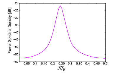Power spectrum of the process generating \(g\)

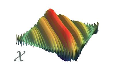Actual correlation matrix of the signal \(x\)

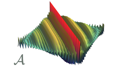Optimal correlation profile for the rows of \(A\)

sensing matrices

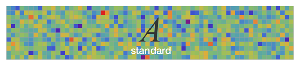
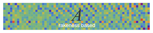
Such signals are acquired by means of two different sensing matrices both with \(m=12\) rows: a matrix \(A\) made of i.i.d. Gaussian zero-mean and unit variance entries, and a matrix \(A\) with independent rows, each of them generated by a multivariate Gaussian distribution with zero mean and a correlation matrix \(\mathcal{A}\) given by the rakeness-based approach (see the above plots). A typical pair of matrices is rendered as colormaps below: visual inspection confirms that the righ-hand matrix has slightly more low-pass rows w.r.t. the left-hand one.

results

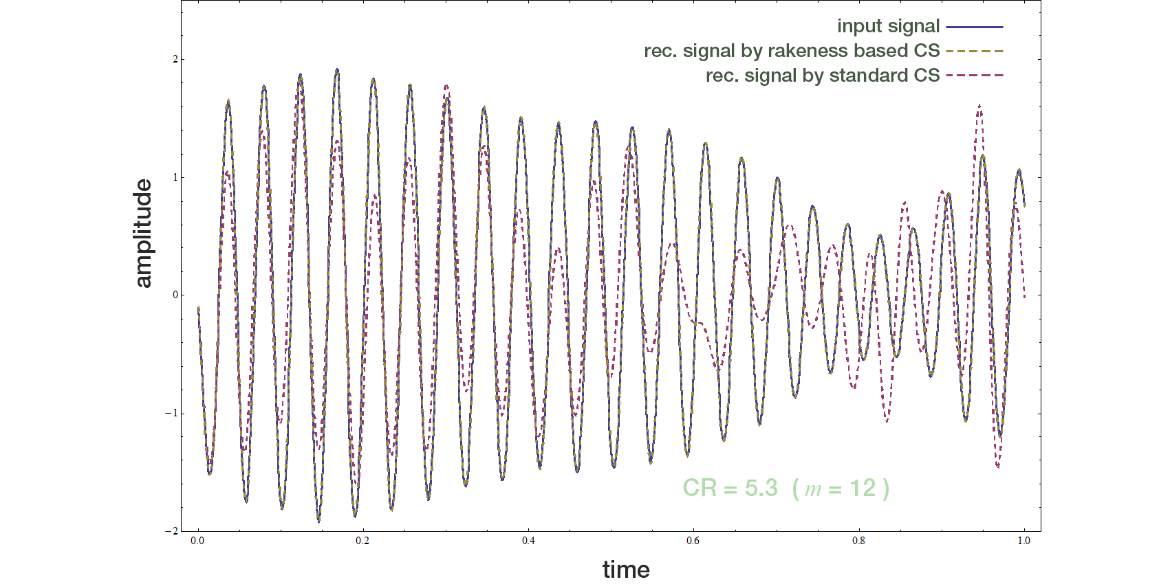
In boh cases, the signal is recovered by solving the the standard \(\min_{l1}\) optimization problem. The reconstructions are reported, along with the input signal, in the next figure. Performance is measured in terms of Reconstruction-SNR (RSNR), i.e., if \(x\) is the true signal and \(\hat{x}\) the one output by te \(\min_{l1}\) optimization, \( \left(RSNR=[||x||_2/||x-\hat{x}||_2]_{dB}\right) \). In this case RSNR=4.1dB for the i.i.d. projection matrix (the one that would have been used by standard CS) and RSNR=40.1dB for the rakeness-based projection matrix.

Though this only implicitly enters the design flow, rakeness-based design assumes that the input signal is localized, i.e., that its energy is not uniformly distributed in the whole signal space so that the correlation matrix \(\mathcal{X}={\mathbf E}[xx^\top]\) is not a multiple of the identity. To quantify localizazion we may measure how much the eigenvalues \(\lambda_j(\mathcal{X})\) for \(j=1,\dots,n\) of \(\mathcal{X}\) deviate from a uniform distribution of the total energy \({\rm tr}(\mathcal{X})\). A straightforward option is $$ \mathfrak{L}_x=\sum_{j=0}^{n-1}\left(\frac{\lambda_j(\mathcal{X})}{\mathrm{tr}(\mathcal{X})}-\frac{1}{n}\right)^2 =\frac{\mathrm{tr}\left(\mathcal{X}^2\right)}{\mathrm{tr}^2(\mathcal{X})}-\frac{1}{n} $$

The above localization measure satisfies \(0\le\mathfrak{L}_x\le 1-\frac{1}{n}\) where the upper bound corresponds to a unique non-zero eigenvalue and thus to a distribution producing vectors along a unique direction identified by the corresponding eigenvector. The lower bound corresponds to an isotropic distribution producing vectors with uncorrelated entries. If \(\mathfrak{L}_x=0\) the solution of the rakeness maximization problem would yield \(\mathcal{A}=\frac{e}{n}\mathcal{I}\) where \(\mathcal{I}\) is the identity matrix and thus, classical i.i.d. sensing would be the optimal choice. Yet, typical real-world signals have \(\mathfrak{L}_x>0\) and the \(\mathcal{A}\) resulting from the rakeness maximization problem achieves better results w.r.t. classical i.i.d. sensing.

Finally, both localization and rakeness depend quadratically on the second-order statistical features of the entailed vectors. This results in a link between the two quantities $$ \mathfrak{L}_a=\frac{\mathrm{tr}\left(\mathcal{A}^2\right)}{\mathrm{tr}^2(\mathcal{A})}-\frac{1}{n}= \frac{\rho(a,a)}{e^2}-\frac{1}{n} $$ and allows to recast the rakeness maximization problem into $$ \begin{array}{ll} \displaystyle \max_{\mathcal{A}} & \;\;\displaystyle \mathrm{tr}(\mathcal{A}\mathcal{X})\\[0.5em] {\rm s.t.} & \begin{array}{l} \mathcal{A}\succeq 0\\ \mathrm{tr}(\mathcal{A})=e\\ \mathfrak{L}_a\le\ell\mathfrak{L}_x \end{array} \end{array} $$ where the randomness constraint giving a cap on \(\rho(a,a)\) is translated in a more intuitive constraint requiring that the sensing waveforms (\(a\)) are localized not more than \(\ell\) times the waveforms they have to sense (\(x\)).

Cambareri, V.; Mangia, M.; Pareschi, F.; Rovatti, R.; Setti, G., "A rakeness-based design flow for Analog-to-Information conversion by Compressive Sensing," Circuits and Systems (ISCAS), 2013 IEEE International Symposium on, pp.1360-1363, 2013 - doi: 10.1109/BioCAS.2011.6107818