Rakeness

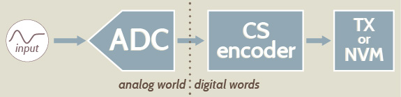
The fact that CS provides a compression w.r.t. the number of Nyquist-rate samples implies that the same real-world quantity can be represented (and thus stored and transmitted) with fewer bits. Since, for example, the transmission data rate directly affects the power consumption of trasmitters, CS is seen as a possible method to design autonomous sensor nodes with a less power-hungry radio interface. Celarly, this happens at the expense of a linear processing (the multiplication by the matrix \(A\)) that though simple does not come for free. Low-power implementations of CS stages are therefore important to administer the trade off between the achieved compression and the resources needed to obtain it. Different paths may be taken depending on whether CS is applied directly in the analog domain or after an initial conventional sampling as a mere compression stage.

In the analog world

CS approach applied directly in the analog domain

• Analog CS

  Analog CS

Working with digital words

CS approach as a compression stage

• Digital CS

  Digital CS

A possible choice to reduce the power consumption of an autonomous sensor node, is to apply CS directly in the analog domain. This yields advantages in terms of both reduction of the amount of transmitted digital words and on the effort due to digital conversion. Some analog CS based solutions have been proposed so far in the Literature (Pareschi et al., Shoaran et al. and Gangopadhyay et al.). All of them are based on the Random Modulation Pre-Integration (RMPI) architecture, which was shown to be the most versatile in terms of capability to acquire signals that are sparse in an arbitrary base.

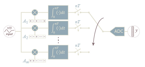
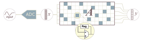
The measurement vector \(y\) is obtained by projecting the analog signal \(x(t)\) over a set of \(m\) sensing functions \(a_j(t)\) characterizing the projecting operator, i.e., \(y_j=\int_{T}a_j(t)x(t)dt\). The values \(y_j\) can be converted into digital form by a shared sub-Nyquist ADC, whose rate is \(m/T\) conversions per time unit, that is smaller with respect to the Nyquist rate \(= n/T\).

The most common implementation of the above processing is by means of a switched-capacitor architecture. This implicitly leads to a discrete time characterization in which the \(m\) measurements are obtained by means of an equivalent matrix-by-vector product \(y_j = \sum_{i=1}^n A_{j,i} x_i\).

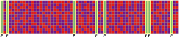
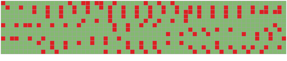
Having that physical implementation in mind, the most convenient way to ensure a correct input signal reconstruction is to generate sensing vectors \(a_j\), as antipodal random vectors, where the two possible values \(+1\) and \(-1\) occurs with the same probability. This relaxes the product operations required to compute the \(m\) projections into much simpler sign inversion operations, and allows a simpler hardware implementation at no costs in terms of CS performance reduction. Fixing a proper reconstruction quality level, a further reduction in terms of minimum value of \(m\) can be reach by the rakeness-based CS w.r.t. the standard CS approach. Its implies an higher compression ratio and less parallel branch in the RMPI architecture. Two possible sensing matrix \(A\) following respectively standard CS and rakeness-based CS are reported below in the case where the input signal is sparse in the DCT basis and it is also localized with a pass-band profile (see the main page, section EXAMPLE  ).

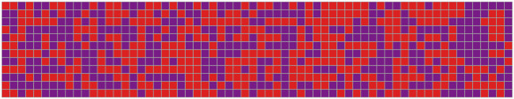
Antipodal i.i.d. sensing matrix

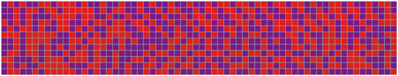
Antipodal localized sensing matrix

F. Pareschi, P. Albertini, G. Frattini, M. Mangia, R. Rovatti and G. Setti, "Hardware-Algorithms Co-design and Implementation of an Analog-to-Information Converter for Biosignals based on Compressed Sensing," IEEE Trans. Biomedical Circuits and Systems, to appear, 2015

M. Shoaran, M. H. Kamal, C. Pollo, P. Vandergheynst, and A. Schmid, “Compact Low-Power Cortical Recording Architecture for Compressive Multichannel Data Acquisition,” IEEE Trans. Biomedical Circuits and Systems, vol. 8, no. 6, pp. 857–870, 2014 - doi: 10.1109/TBCAS.2014.2304582

D. Gangopadhyay, E. Allstot, A. Dixon, K. Natarajan, S. Gupta, and D. Allstot, “Compressed Sensing Analog Front-End for Bio-Sensor Applications,” IEEE Journal of Solid-State Circuits, vol. 49, no. 2, pp. 426–438, 2014 - doi: 10.1109/JSSC.2013.2284673

In principle, the computation of \(y=Ax\) where \(x\in\mathbb{R}^n\) and \(A\) is \(m\times n\) entails \(\mathcal{O}(nm)\) multiplications and sums. When \(n\) and consequently \(m\) increase, such a computational burden may correspond to a significant power consumption that at least partially compensates the gain due to the compression \(m\lt n\).

There are two features of \(A\) that may help reducing such a burden: the fact that \(A\) is sparse, i.e., many of its entries are null, the fact of non-null entries in \(A\) can be encoded with a very small number of bits.

The fact that many entries are zero implies that the whole corresponding multiply-and-accumulate operations can be dropped. The adoption of low-depth values for the non-null elements of \(A\) implies that the multipliers needed in the linear combination can be very simple to the limit of being substituted by a simple signed sum when the entries are either \(+1\) or \(-1\)). Overall, this suggests that \(A\) is either a ternary \(A_{i,j}\in\{-1,0,+1\}\) or binary \(A_{i,j}\in\{0,1\}\) matrix.

In this case \(A_{i,j}\in\{-1,0,+1\}\) and this has some consequences on the features of \(\mathcal{A}\) that must be possessed by the solution of the rakeness problem. In particular, for any entry \(a_i\) of a row of \(A\) we have \(\mathbf{E}[a^2_i]=\Pr\{a_i\neq 0\}\). Hence, \(\mathcal{A}_{i,i}\) is equal to the probability that the \(i\)-th entry is non-null. Moreover, it must also be \(|\mathcal{A}_{i,j}|=|\mathbf{E}[a_ia_j]|\le\min\{\Pr\{a_i\neq 0\},\Pr\{a_j\neq 0\}\}=\min\{\mathcal{A}_{i,i},\mathcal{A}_{j,j}\}\) that adds to the natural \(\mathcal{A}\succeq 0\).

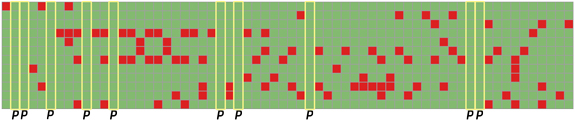
Further to that, zeros may be distributed in the matrix according to policies with different potential impact on the implementation.

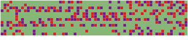
A first policy is puncturing and its effects are reported in the figure below. Entire columns of \(A\) are zeroed. Thugh this may typically have a non-negligible effect on the subsequent reconstruction, it has the advantage of making certain samples of \(x\) (those corresponding to zeroed columns) unnecessary. Hence, sampling and even the pre-sampling analog processing (e.g., the typical anti-aliasing filter) may be left idle or switched off (if the sampling frequency is low enough w.r.t. the internal circuit dynamics) for the entire sample time.

A second policy is throttling that zeroes the same number of entires in each column even if in different positions. With this, the number of nonzeros is also fixed meaning that each time a sample comes in, a reduced and pre-determined number of multiply-and-accumulate operations (signed sums in our case) are needed. Throttling so that only \(t\lt m\) entries are non-zero in each column means reducing the effort needed to compute the product by an \(m\times n\) matrix to that of computing the product by a \(t\times n\) matrix.

Obviously both puncturing and throttling can be applied simultaneously.

Puncturing

Throttling

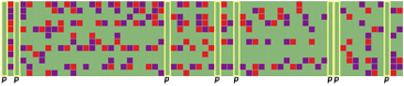
Puncturing & Throttling

Since zeroing elements in \(A\) means that the computation of the measurements \(y=Ax\) has less chances to look at the signal \(x\), the remaining chances must be carefully administered and this is what a suitably modified rakeness-based approach is able to do.

In this case \(A_{i,j}\in\{0,1\}\) and, while the interpretation of the diagonal elements of \(\mathcal{A}\) as the probability of non-zero still holds, the bound of the non-diagonal elements changes into \(\max\{0,\mathcal{A}_{i,i}+\mathcal{A}_{j,j}-1\}\le \mathcal{A}_{i,j}\le \min\{\mathcal{A}_{i,i},\mathcal{A}_{j,j}\}\).

For binary matrices, setting zeros is equivalent to setting non-zeros. Both puncturing and throttling can be applied though the absence of \(-1\) entries in \(A\) usually leads to lower performance for the same number of non-zero entries.

Throttling

Puncturing & Throttling

F. Pareschi, V. Cambareri, R. Rovatti, G. Setti, ''Rakeness-Based Design of Low-Complexity Compressed Sensing'', IEEE Transactions on Circuits and Systems I: Regular Papers, vol. 64, no. 5, pp. 1201-1213, 2017 - doi: 10.1109/TCSI.2017.2649572