Rakeness-based CS with Matlab
The starting piece of information on which rakeness-based design hinges is the correlation matrix of the vector to acquire \(\mathcal{X}=\mathbf{E}[xx^\top]\). If such a matrix is not known from a-priori considerations, it may be estimated from known instances of \(x\). If the number \(s\) of known instances \(x_1,x_2,\dots,x_s\) is large enough, one may resort to a trivial estimation by means of the sample correlation matrix $$ \mathcal{X}\simeq\frac{1}{s}\sum_{i=1}^{s}x_ix_i^\top $$
The following Matlab code reports the estimation of the correlation matrix of a synthetic sparse and localized signal in the DCT basis with a band pass (BP) profile (see the main page, section EXAMPLE ). The final estimation is represented by the variable KX.
% System setting
n = 64; % dimensionality of the signal to acquire
k = 6; % sparsity of the signal to acquire
% Estimation of the correlation matrix of the signal to acquire
x = GenSyn(n,k,10000,'BP','Fourier'); % 10.000 random instances are generated
KX = x*x'/10000; % estimated correlation matrix
Once that the correlation matrix is known and if no constraint is put on the elements of the sensing matrix \(A\), one may proceed to the analytical solution of the "rakeness problem" with a randomness constraint \(l\mathfrak{L}_x\) and a given energy \(e\) for the rows of \(A\). The solution of such a problem gives the correlation matrix \(\mathcal{A}\) (KA in the code) that should control the generation of the rows of \(A\) (see the main page, section MORE DETAILS ).
In the following the Matlab code to obtain at first the desidered correlation matrix (with \(e=1\) and \(l=0.5\)) and then each row of \(A\) is generated as instance of a multivariate Gaussian distribution with zero mean and a correlation matrix KA.
e = 1; % energy of each row of A
ell = 0.5; % randomness constraint
KA = Rak(KX,e,ell); % solve rakeness problem
m = 20; % number of rows in A
A = Gen(KA,m); % generation of A
This \(A\) allows the acquisition and reconstruction of new instances of the signal. In the following Matlab code, reconstruction is done by solving the \(\min_{l1}\) optimization problem using the solver named SPGL1. A typical result of such a reconstruction is shown in the main page, section EXAMPLE .
[x, S] = GenSyn(n,k,1,'BP','Fourier'); %signal instance and sparsity matrix
y = A*x; % sensing stage
xr = S*spgl1(A*S,y); % decoding stage
As described in the low-power page (section DIGITAL CS ), the resourced needed for to compute \(y=Ax\) can be reduced by putting constraints on the matrix \(A\). In particular, antipodal, ternary or binary matrices are the most parsimonious choices and zeroes in \(A\) actually translate in a reduction of the number of multiply-and-accumulate operations.
In these cases the rakeness problem must be solved taking into account additional constraints depending on the matrix type. Such constraints prevent an analytical solution and call for convex numerical optimization methods. The functions we provide adopt the projected-gradient approach (see Goldstein for more details).
Once that \(\mathcal{A}\) is computed, a last problem must be addressed, i.e., that of generating vectors with a prescribed correlation profile whose entries can be only \(-1,0,+1\). The functions we provide solve this problem generalizing a classical method derived from the considerations of Van Vleck et al. on clipped Gaussian noise.
Overall there are three steps to be taken, the first two of which can be performed off-line,
- Starting from \(\mathcal{X}\), solve rakeness optimization problem with additional constraints and obtain \(\mathcal{A}\)
- Starting from \(\mathcal{A}\), pre-compute the parameters of the matrix generator.
- Use the generator to generate the matrix \(A\) needed for acquisition.
For each of these steps there is a function whose use we detail in the following.
A.A. Goldstein, "Convex Programming in Hilbert Space," Bullettin of the American Mathematical Society, vol. 70, pp. 709-710, 1964
J.H. Van Vleck, D. Middleton, "The Spectrum of Clipped Noise," IEEE Proceedings, vol.54, no.1, pp.2-19, 1966 - doi: 10.1109/PROC.1966.4567
Antipodal & Ternary matrix
KA = TRak(KX,eta,ell)
Binary matrix
KA = BRak(KX,eta,ell)
These two functions solve the rakeness problem starting from \(\mathcal{X}\) (KX in the code). The second argument eta corresponds to the diagonal of the matrix \(\mathcal{A}\) that will be produced (KA in the code) and controls the average number of non-zeros in the corresponding position of the generated vectors. Hence, if the i-th element of eta equal to zero, then \(\mathcal{A}_{i,i}=0\) and thus all the rows of \(A\) will be zero in that position. If, on the contrary, the same element is 1 then \(\mathcal{A}_{i,i}=1\) and all the rows of \(A\) will be non-zero in that position. The last argument ell bounds the localization of the sensing vectors (ell is typically set at 0.5).
Antipodal & Ternary matrix
[KG th] = TGau(KA)
Binary matrix
[KG th] = BGau(KA)
These functions generate the \(n\times n\) matrix KG and the \(n\times 1\) vector th that are needed by the generator of the rows of \(A\) to produce vectors whose correlation is as close as possible to \(\mathcal{A}\) and whose values are constrained either in \(\{-1,0,1\}\) or in \(\{0,1\}\).
Antipodal & Ternary matrix
A = TGen(KG,th,m)
Binary matrix
A = BGen(KG,th,m)
These functions generate the \(m\times n\) sensing matrix A composed by m properly generated rows.
While the first two steps can be performed offline, this last step should be repeted every time a different instance of the acquisition matrix is needed, i.e., potentially every time a new vector \(x\) must be sensed, though in many applications a fixed typical instance of \(A\) is enough to deliver satisfactory results.
Matlab examples
Antipodal matrix
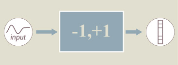
Antipodal matrix are tipically used in the design of analog devices implementing rakeness-based CS as an analog-to-digital converter.
Ternary matrix
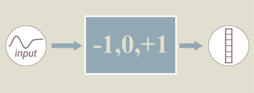
Ternay matrix are tipically used in the digital domain where rakeness-based CS acts as a lightweight compression stage.
Binary matrix
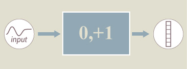
Binary matrix are used as an extremely lightweight option in both the analog-to-digital conversion case and in the digital compression case.
Antipodal Matrices
CR = 3; % compression ratio
m = round(n/CR); % number of rows in A
eta = ones(n,1); % A must be antipodal
ell = 0.5; % bound on sensing localization
% Solve the rakeness problem
KA = TRak(KX,eta,ell);
% Compute the generator parameters
[KG th] = TGau(KA);
% Generate A
A = TGen(KG,th,m);
Ternary Matrices
Puncturing
CR = 3; % compression ratio
PR = 3; % puncturing ratio
nc = round(n*(PR-1)/PR); % number of zeroed columns in A
indp = randperm(n,nc); % indexes of zeroed columns
m = round(n/CR); % number of rows in A
eta = ones(n,1); % A is zeroed only by puncturing
eta(indp) = 0;
ell = 0.5; % bound on sensing localization
% Solve the rakeness problem
KA = TRak(KX,eta,ell);
% Compute the generator parameters
[KG th] = TGau(KA);
% Generate A
A = TGen(KG,th,m);
Throttling
CR = 3; % compression ratio
AT = 0.25; % average throttling
m = round(n/CR); % number of rows in the sensing matrix
p = (m*AT)^-1; % probability of a non-zero entry
eta = p*ones(n,1);
ell = 0.5; % bound on sensing localization
% Solve the rakeness problem
KA = TRak(KX,eta,ell);
% Compute generator parameters
[KG th] = TGau(KA);
% Generate A
maxIter = 1000;
loop = true;
iter = 0;
while loop
A = TGen(KG,th,m);
czero = sum(sum(abs(A))==0);
rzero = sum(sum(abs(A'))==0);
% to prevents unwanted null columns/rows that may appear for large values of AT
if iter>=maxIter || (czero==0 && rzero==0)
loop=false;
end
iter = iter+1;
end
Puncturing & Throttling
CR = 3; % compression ratio
PR = 1.1; % puncturing ratio
AT = 0.25; % average throttling
nc = round(n*(PR-1)/PR); % number of zeroed columns in A
indp = randperm(n,nc); % indexes of zeroed columns
m = round(n/CR); % number of rows in A
p = (m*AT)^-1; % probability of a non-zero entry in non-zeroed columns
eta = p*ones(n,1);
eta(indp) = 0;
ell = 0.5; % bound on sensing localization
% Solve the rakeness problem
KA = TRak(KX,eta,ell);
% Compute generator parameters
[KG th] = TGau(KA);
% Generate A
maxIter = 1000;
loop = true;
iter = 0;
while loop
A = TGen(KG,th,m);
czero = sum(sum(abs(A))==0);
rzero = sum(sum(abs(A'))==0);
% to prevents unwanted null columns/rows that may appear for large values of AT
if iter>=maxIter || (czero==nc && rzero==0)
loop=false;
end
iter = iter+1;
end
Binary matrices
Throttling
CR = 3; % compression ratio
AT = 0.25; % average throttling
m = round(n/CR); % amount of rows in the sensing matrix
p = (m*AT)^-1; % probability of a non-zero entry
eta = p*ones(n,1);
ell = 0.5; % bound on sensing localization
% Solve the rakeness problem
KA = BRak(KX,eta,ell);
% Compute generator parameters
[KG th] = BGau(KA);
% Generate A
maxIter = 1000;
loop = true;
iter = 0;
while loop
A = BGen(KG,th,m);
czero = sum(sum(abs(A))==0);
rzero = sum(sum(abs(A'))==0);
% to prevents unwanted null columns/rows that may appear for large values of AT
if iter>=maxIter || ( czero==0 && rzero==0)
loop=false;
end
iter = iter+1;
end
Puncturing & Throttling
CR = 3; % compression ratio
PR = 1.1; % puncturing ratio
AT = 0.25; % average throttling
nc = round(n*(PR-1)/PR); % number of zeroed columns in A
indp = randperm(n,nc); % indexes of columns to be zeroed
m = round(n/CR); % number of rows in A
p = (m*AT)^-1; % probablity to have non-zero entry in each non-zeroed column
eta = p*ones(n,1);
eta(indp) = 0;
ell = 0.5; % bound on sensing localization
% Solve the rakeness problem
KA = BRak(KX,eta,ell);
% Compute generator parameters
[KG th] = BGau(KA);
% Generate A
maxIter = 1000;
loop = true;
iter = 0;
while loop
A = BGen(KG,th,m);
czero = sum(sum(abs(A))==0);
rzero = sum(sum(abs(A'))==0);
% to prevents unwanted null columns/rows that may appear for large values of AT
if iter>=maxIter || (czero==nc && rzero==0)
loop=false;
end
iter = iter+1;
end